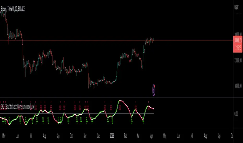
GKD-C Blau Stochastic Momentum Index [Loxx]Giga Kaleidoscope GKD-C Blau Stochastic Momentum Index is a Confirmation module included in Loxx's "Giga Kaleidoscope Modularized Trading System".
█ Giga Kaleidoscope Modularized Trading System
What is Loxx's "Giga Kaleidoscope Modularized Trading System"?
The Giga Kaleidoscope Modularized Trading System is a trading system built on the philosophy of the NNFX (No Nonsense Forex) algorithmic trading.
What is the NNFX algorithmic trading strategy?
The NNFX (No-Nonsense Forex) trading system is a comprehensive approach to Forex trading that is designed to simplify the process and remove the confusion and complexity that often surrounds trading. The system was developed by a Forex trader who goes by the pseudonym "VP" and has gained a significant following in the Forex community.
The NNFX trading system is based on a set of rules and guidelines that help traders make objective and informed decisions. These rules cover all aspects of trading, including market analysis, trade entry, stop loss placement, and trade management.
Here are the main components of the NNFX trading system:
1. Trading Philosophy: The NNFX trading system is based on the idea that successful trading requires a comprehensive understanding of the market, objective analysis, and strict risk management. The system aims to remove subjective elements from trading and focuses on objective rules and guidelines.
2. Technical Analysis: The NNFX trading system relies heavily on technical analysis and uses a range of indicators to identify high-probability trading opportunities. The system uses a combination of trend-following and mean-reverting strategies to identify trades.
3. Market Structure: The NNFX trading system emphasizes the importance of understanding the market structure, including price action, support and resistance levels, and market cycles. The system uses a range of tools to identify the market structure, including trend lines, channels, and moving averages.
4. Trade Entry: The NNFX trading system has strict rules for trade entry. The system uses a combination of technical indicators to identify high-probability trades, and traders must meet specific criteria to enter a trade.
5. Stop Loss Placement: The NNFX trading system places a significant emphasis on risk management and requires traders to place a stop loss order on every trade. The system uses a combination of technical analysis and market structure to determine the appropriate stop loss level.
6. Trade Management: The NNFX trading system has specific rules for managing open trades. The system aims to minimize risk and maximize profit by using a combination of trailing stops, take profit levels, and position sizing.
Overall, the NNFX trading system is designed to be a straightforward and easy-to-follow approach to Forex trading that can be applied by traders of all skill levels.
Core components of an NNFX algorithmic trading strategy
The NNFX algorithm is built on the principles of trend, momentum, and volatility. There are six core components in the NNFX trading algorithm:
1. Volatility - price volatility; e.g., Average True Range, True Range Double, Close-to-Close, etc.
2. Baseline - a moving average to identify price trend
3. Confirmation 1 - a technical indicator used to identify trends
4. Confirmation 2 - a technical indicator used to identify trends
5. Continuation - a technical indicator used to identify trends
6. Volatility/Volume - a technical indicator used to identify volatility/volume breakouts/breakdown
7. Exit - a technical indicator used to determine when a trend is exhausted
What is Volatility in the NNFX trading system?
In the NNFX (No Nonsense Forex) trading system, ATR (Average True Range) is typically used to measure the volatility of an asset. It is used as a part of the system to help determine the appropriate stop loss and take profit levels for a trade. ATR is calculated by taking the average of the true range values over a specified period.
True range is calculated as the maximum of the following values:
-Current high minus the current low
-Absolute value of the current high minus the previous close
-Absolute value of the current low minus the previous close
ATR is a dynamic indicator that changes with changes in volatility. As volatility increases, the value of ATR increases, and as volatility decreases, the value of ATR decreases. By using ATR in NNFX system, traders can adjust their stop loss and take profit levels according to the volatility of the asset being traded. This helps to ensure that the trade is given enough room to move, while also minimizing potential losses.
Other types of volatility include True Range Double (TRD), Close-to-Close, and Garman-Klass
What is a Baseline indicator?
The baseline is essentially a moving average, and is used to determine the overall direction of the market.
The baseline in the NNFX system is used to filter out trades that are not in line with the long-term trend of the market. The baseline is plotted on the chart along with other indicators, such as the Moving Average (MA), the Relative Strength Index (RSI), and the Average True Range (ATR).
Trades are only taken when the price is in the same direction as the baseline. For example, if the baseline is sloping upwards, only long trades are taken, and if the baseline is sloping downwards, only short trades are taken. This approach helps to ensure that trades are in line with the overall trend of the market, and reduces the risk of entering trades that are likely to fail.
By using a baseline in the NNFX system, traders can have a clear reference point for determining the overall trend of the market, and can make more informed trading decisions. The baseline helps to filter out noise and false signals, and ensures that trades are taken in the direction of the long-term trend.
What is a Confirmation indicator?
Confirmation indicators are technical indicators that are used to confirm the signals generated by primary indicators. Primary indicators are the core indicators used in the NNFX system, such as the Average True Range (ATR), the Moving Average (MA), and the Relative Strength Index (RSI).
The purpose of the confirmation indicators is to reduce false signals and improve the accuracy of the trading system. They are designed to confirm the signals generated by the primary indicators by providing additional information about the strength and direction of the trend.
Some examples of confirmation indicators that may be used in the NNFX system include the Bollinger Bands, the MACD (Moving Average Convergence Divergence), and the MACD Oscillator. These indicators can provide information about the volatility, momentum, and trend strength of the market, and can be used to confirm the signals generated by the primary indicators.
In the NNFX system, confirmation indicators are used in combination with primary indicators and other filters to create a trading system that is robust and reliable. By using multiple indicators to confirm trading signals, the system aims to reduce the risk of false signals and improve the overall profitability of the trades.
What is a Continuation indicator?
In the NNFX (No Nonsense Forex) trading system, a continuation indicator is a technical indicator that is used to confirm a current trend and predict that the trend is likely to continue in the same direction. A continuation indicator is typically used in conjunction with other indicators in the system, such as a baseline indicator, to provide a comprehensive trading strategy.
What is a Volatility/Volume indicator?
Volume indicators, such as the On Balance Volume (OBV), the Chaikin Money Flow (CMF), or the Volume Price Trend (VPT), are used to measure the amount of buying and selling activity in a market. They are based on the trading volume of the market, and can provide information about the strength of the trend. In the NNFX system, volume indicators are used to confirm trading signals generated by the Moving Average and the Relative Strength Index. Volatility indicators include Average Direction Index, Waddah Attar, and Volatility Ratio. In the NNFX trading system, volatility is a proxy for volume and vice versa.
By using volume indicators as confirmation tools, the NNFX trading system aims to reduce the risk of false signals and improve the overall profitability of trades. These indicators can provide additional information about the market that is not captured by the primary indicators, and can help traders to make more informed trading decisions. In addition, volume indicators can be used to identify potential changes in market trends and to confirm the strength of price movements.
What is an Exit indicator?
The exit indicator is used in conjunction with other indicators in the system, such as the Moving Average (MA), the Relative Strength Index (RSI), and the Average True Range (ATR), to provide a comprehensive trading strategy.
The exit indicator in the NNFX system can be any technical indicator that is deemed effective at identifying optimal exit points. Examples of exit indicators that are commonly used include the Parabolic SAR, the Average Directional Index (ADX), and the Chandelier Exit.
The purpose of the exit indicator is to identify when a trend is likely to reverse or when the market conditions have changed, signaling the need to exit a trade. By using an exit indicator, traders can manage their risk and prevent significant losses.
In the NNFX system, the exit indicator is used in conjunction with a stop loss and a take profit order to maximize profits and minimize losses. The stop loss order is used to limit the amount of loss that can be incurred if the trade goes against the trader, while the take profit order is used to lock in profits when the trade is moving in the trader's favor.
Overall, the use of an exit indicator in the NNFX trading system is an important component of a comprehensive trading strategy. It allows traders to manage their risk effectively and improve the profitability of their trades by exiting at the right time.
How does Loxx's GKD (Giga Kaleidoscope Modularized Trading System) implement the NNFX algorithm outlined above?
Loxx's GKD v1.0 system has five types of modules (indicators/strategies). These modules are:
1. GKD-BT - Backtesting module (Volatility, Number 1 in the NNFX algorithm)
2. GKD-B - Baseline module (Baseline and Volatility/Volume, Numbers 1 and 2 in the NNFX algorithm)
3. GKD-C - Confirmation 1/2 and Continuation module (Confirmation 1/2 and Continuation, Numbers 3, 4, and 5 in the NNFX algorithm)
4. GKD-V - Volatility/Volume module (Confirmation 1/2, Number 6 in the NNFX algorithm)
5. GKD-E - Exit module (Exit, Number 7 in the NNFX algorithm)
(additional module types will added in future releases)
Each module interacts with every module by passing data between modules. Data is passed between each module as described below:
GKD-B => GKD-V => GKD-C(1) => GKD-C(2) => GKD-C(Continuation) => GKD-E => GKD-BT
That is, the Baseline indicator passes its data to Volatility/Volume. The Volatility/Volume indicator passes its values to the Confirmation 1 indicator. The Confirmation 1 indicator passes its values to the Confirmation 2 indicator. The Confirmation 2 indicator passes its values to the Continuation indicator. The Continuation indicator passes its values to the Exit indicator, and finally, the Exit indicator passes its values to the Backtest strategy.
This chaining of indicators requires that each module conform to Loxx's GKD protocol, therefore allowing for the testing of every possible combination of technical indicators that make up the six components of the NNFX algorithm.
What does the application of the GKD trading system look like?
Example trading system:
Backtest: Strategy with 1-3 take profits, trailing stop loss, multiple types of PnL volatility, and 2 backtesting styles
Baseline: Hull Moving Average
Volatility/Volume: Hurst Exponent
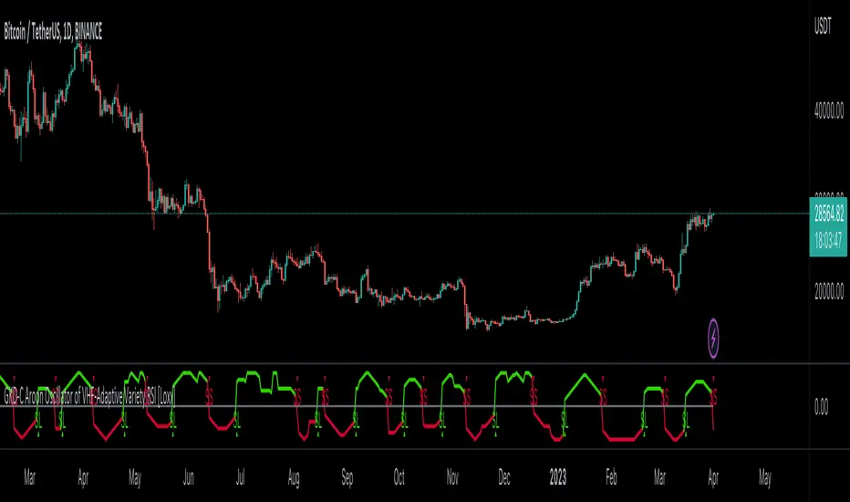
Confirmation 1: Blau Stochastic Momentum Index as shown on the chart above
Confirmation 2: Williams Percent Range
Continuation: Fisher Transform
Exit: Rex Oscillator
Each GKD indicator is denoted with a module identifier of either: GKD-BT, GKD-B, GKD-C, GKD-V, or GKD-E. This allows traders to understand to which module each indicator belongs and where each indicator fits into the GKD protocol chain.
Giga Kaleidoscope Modularized Trading System Signals (based on the NNFX algorithm)
Standard Entry
1. GKD-C Confirmation 1 Signal
2. GKD-B Baseline agrees
3. Price is within a range of 0.2x Volatility and 1.0x Volatility of the Goldie Locks Mean
4. GKD-C Confirmation 2 agrees
5. GKD-V Volatility/Volume agrees
Baseline Entry
1. GKD-B Baseline signal
2. GKD-C Confirmation 1 agrees
3. Price is within a range of 0.2x Volatility and 1.0x Volatility of the Goldie Locks Mean
4. GKD-C Confirmation 2 agrees
5. GKD-V Volatility/Volume agrees
6. GKD-C Confirmation 1 signal was less than 7 candles prior
Continuation Entry
1. Standard Entry, Baseline Entry, or Pullback; entry triggered previously
2. GKD-B Baseline hasn't crossed since entry signal trigger
3. GKD-C Confirmation Continuation Indicator signals
4. GKD-C Confirmation 1 agrees
5. GKD-B Baseline agrees
6. GKD-C Confirmation 2 agrees
1-Candle Rule Standard Entry
1. GKD-C Confirmation 1 signal
2. GKD-B Baseline agrees
3. Price is within a range of 0.2x Volatility and 1.0x Volatility of the Goldie Locks Mean
Next Candle:
1. Price retraced (Long: close < close or Short: close > close )
2. GKD-B Baseline agrees
3. GKD-C Confirmation 1 agrees
4. GKD-C Confirmation 2 agrees
5. GKD-V Volatility/Volume agrees
1-Candle Rule Baseline Entry
1. GKD-B Baseline signal
2. GKD-C Confirmation 1 agrees
3. Price is within a range of 0.2x Volatility and 1.0x Volatility of the Goldie Locks Mean
4. GKD-C Confirmation 1 signal was less than 7 candles prior
Next Candle:
1. Price retraced (Long: close < close or Short: close > close )
2. GKD-B Baseline agrees
3. GKD-C Confirmation 1 agrees
4. GKD-C Confirmation 2 agrees
5. GKD-V Volatility/Volume Agrees
PullBack Entry
1. GKD-B Baseline signal
2. GKD-C Confirmation 1 agrees
3. Price is beyond 1.0x Volatility of Baseline
Next Candle:
1. Price is within a range of 0.2x Volatility and 1.0x Volatility of the Goldie Locks Mean
3. GKD-C Confirmation 1 agrees
4. GKD-C Confirmation 2 agrees
5. GKD-V Volatility/Volume Agrees
█ GKD-C Blau Stochastic Momentum Index
What is Blau Stochastic Momentum Index?
The Blau Stochastic Momentum Index (BSMI) is a technical analysis indicator used to measure momentum in financial markets. It was developed by William Blau, a well-known trader and author of several books on technical analysis.
The BSMI is based on the Stochastic Momentum Index (SMI), which is a popular momentum indicator that measures the distance between the current closing price and the recent high or low. The SMI is similar to the Stochastic Oscillator, but it takes into account the rate of change in the market, making it more responsive to short-term changes in momentum.
The BSMI is designed to provide a more accurate and responsive measure of momentum than the SMI. It uses a digital signal processing technique called "smoothed moving averages" to filter out noise and provide a smoother, more stable indicator. This technique helps to reduce false signals and provide a clearer picture of market momentum.
The BSMI indicator is plotted on a chart as a line that oscillates between -100 and +100. Values above zero indicate bullish momentum, while values below zero indicate bearish momentum. The BSMI line is typically plotted alongside the price chart to help traders identify potential turning points in the market.
Traders can use the BSMI indicator in a variety of ways, including:
1. Identifying overbought and oversold conditions: When the BSMI line reaches extreme values (e.g., above +80 or below -80), it may indicate that the market is overbought or oversold and due for a reversal.
2. Confirming trend strength: When the BSMI line is trending in the same direction as the price, it can confirm the strength of the trend and help traders stay in winning positions.
3. Identifying divergences: When the BSMI line and the price chart are moving in opposite directions, it may indicate a potential trend reversal or weakening of the current trend.
As with any technical indicator, it is important to use the BSMI in conjunction with other forms of analysis and risk management strategies. No single indicator can predict market movements with 100% accuracy, and traders should always use caution and discipline when making trading decisions.
Requirements
Inputs
Confirmation 1 and Solo Confirmation: GKD-V Volatility / Volume indicator
Confirmation 2: GKD-C Confirmation indicator
Outputs
Confirmation 2 and Solo Confirmation Complex: GKD-E Exit indicator
Confirmation 1: GKD-C Confirmation indicator
Continuation: GKD-E Exit indicator
Solo Confirmation Simple: GKD-BT Backtest strategy
Additional features will be added in future releases.
אינדיקטור Pine Script®